Last year, I implemented the Ray Tracing in One Weekend tutorial in Rust but the rendering was painfully slow on my machine. Instead of adding parallelization to my Rust code, I decided to rewrite my ray tracer again in JAX to get really good performance gains without too much effort.
Ray tracing is an ideal JAX application: it’s computationally intensive but parallel (each pixel is independent), mathematically heavy (lots of vector operations and intersections), and benefits enormously from differentiation for techniques like inverse rendering and neural radiance fields. The pure function nature of ray tracing algorithms (i.e. given a ray and scene, it always produces the same color) also aligns well with JAX’s constraints.
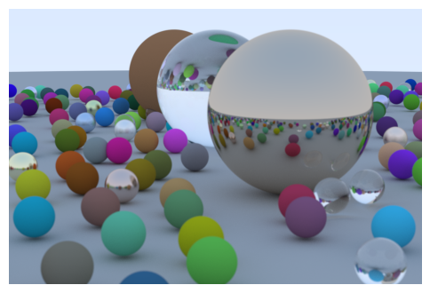
This guide has four parts and ultimately builds up to the iconic Ray Tracer image you see above. I didn’t go super in-depth into all the math/intuition behind each function because it’s all covered in the OG Ray Tracing tutorial, but I tried to map which chapters map to what section. If you want to follow along with runnable code (or make any modifications/extensions), I put it all in this Colab.
*Note: There are some parts in this post where I skip over going through certain redundant code snippets — particularly whenever I need to make a slightly different trace_pixel or render function. You can see the full implementations in Colab.
Part 1: JAX Basics + Single Sphere
Roughly covers Ch. 3: Color rendering; Ch. 4: Rays, a Simple Camera, and Background; Ch. 5: Adding a Sphere; and the start of Ch. 6: Surface Normals.
Imports and setup:
!pip install "jax[cuda12]"
import jax
import jax.numpy as jnp
import numpy as np
import matplotlib.pyplot as plt
from jax import jit, vmap, grad
import time

print("JAX devices:", jax.devices())
Ray Definition
A ray is defined by an origin and a direction: P(t) = A + tb. All ray tracers have a notion of a ray (usually a ray class) and color computation along a ray.
In Rust, we would define Ray as a struct:
pub struct Ray {
    origin: Vec3,
    direction: Vec3
}
However, JAX works best with functional programming and pure functions. Objects with methods can interfere with JAX’s transformations like jit, vmap, and grad. For optimal performance in JAX, we’ll represent rays using separate arrays to pass into functions:
ray_origin = jnp.array([0.0, 0.0, 0.0])
ray_direction = jnp.array([0.0, 0.0, -1.0])

def ray_at(origin, direction, t):
    """Returns the point at parameter t along the ray"""
    return origin + t * direction
Ray-sphere intersection
This function returns whether the ray intersects the sphere and where, solving for t in the ray equation: r(t) = origin + t * direction.
In the Rust hit function, we simply early return if there’s no intersection:
let discriminant = h * h - a * c;
if discriminant < 0.0 {
    return false;
}
But JAX needs to trace through your entire function to understand the computation graph. Early returns create dynamic control flow that depend on runtime, which JAX can’t compile efficiently or differentiate through. Thus, we always do computation but use jnp.where() to mask the results based on the hit condition. *Note: The calculations for the quadratic equation coefficients in the code implementation are simplified: math here.
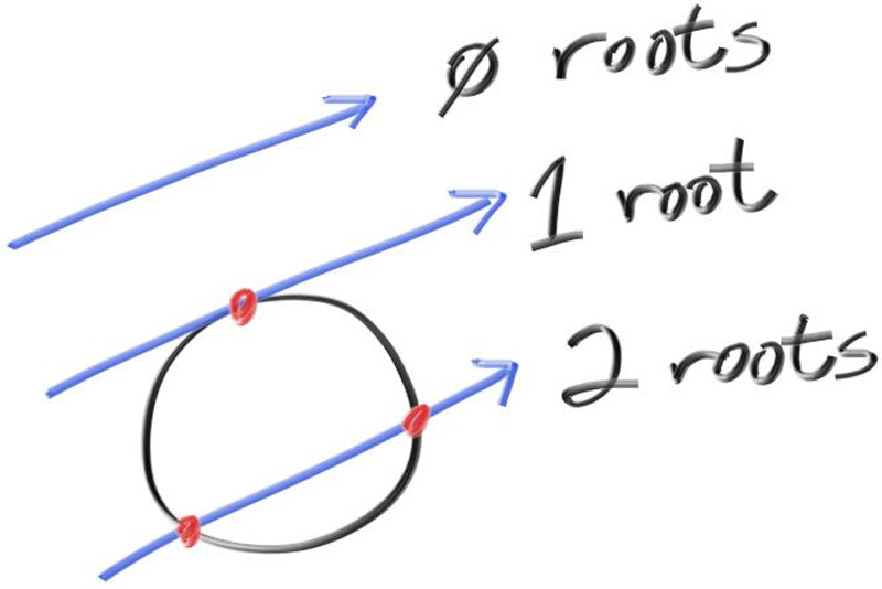
Another example of this jnp.where() JAX hack is root calculation, e.g. the orignal Rust implementation:
// Find the nearest root that lies in the acceptable range
let mut root = (h - sqrt_d) / a; // near root
if !ray_t.surrounds(root) {
    root = (h + sqrt_d) / a; // far root
    if !ray_t.surrounds(root) {
        return false;
    }
}
The far root is often used for implementing refractions (like glass), which needs both entry and exit points – the near and far roots, respectively. (Most of the time, we only use the near root so I was considering just simplifying this code by ignoring the far root completely but I decided that I wanted materials like glass in the final product.)
def ray_sphere_intersect(ray_origin, ray_direction, sphere_center, radius):
  """If and where a ray hits a sphere"""

  # vector from ray origin to sphere center
  oc = sphere_center - ray_origin

  # quadratic equation coeffs
  a = jnp.dot(ray_direction, ray_direction)
  h = jnp.dot(ray_direction, oc)
  c = jnp.dot(oc, oc) - radius * radius

  discriminant = h * h - a * c

  # instead of early return, compute everything but mask results
  hit = discriminant >= 0

  sqrt_d = jnp.sqrt(jnp.maximum(discriminant, 0))
  root_near = (h - sqrt_d) / a
  root_far = (h + sqrt_d) / a

  # Choose the closest positive root
  t = jnp.where(
      root_near > 0,
      root_near,
      jnp.where(root_far > 0, root_far, jnp.inf)
  )

  t = jnp.where(hit, t, jnp.inf)
  p = ray_at(ray_origin, ray_direction, t) # hit point
  outward_normal = (p - sphere_center) / radius
  normal = jnp.where(hit, outward_normal, jnp.zeros(3))

  return hit, t, p, normal
Simple Camera
JAX’s functional programming paradigm means no self or global state. Instead of initializing camera properties once (as you would in Rust’s Camera::new()), we recalculate these “camera constants” each time in camera_get_ray(). While this might seem inefficient, JAX’s JIT compiler is smart enough to optimize these repeated calculations.
Function signatures can sometimes get pretty length in JAX since many individual parameters are passed instead of a single camera struct. This is pretty clunky compared to Rust’s &self, but JAX’s JIT compiler optimizes much better when it sees individual arrays rather than nested Python dictionaries or objects.
The camera viewport represents the 3D plane we’re projecting our 2D image onto. Our goal is transforming pixel coordinates (ranging from 0 to width-1, 0 to height-1) into world space coordinates on this viewport plane.
def create_camera(image_width, image_height):
  """Setup a simple camera"""
  aspect_ratio = image_width / image_height

  # viewport dimensions
  focal_length = 1.0
  viewport_height = 2.0
  viewport_width = viewport_height * (image_width / image_height)
  camera_center = jnp.array([0.0, 0.0, 0.0])

  # viewport vectors
  viewport_u = jnp.array([viewport_width, 0, 0]) # right edge
  viewport_v = jnp.array([0, -viewport_height, 0]) # down edge

  # delta vectors from pixel to pixel
  pixel_delta_u = viewport_u / image_width
  pixel_delta_v = viewport_v / image_height

  # upper left and center pixels
  viewport_upper_left = (camera_center -
                        jnp.array([0, 0, focal_length]) -
                        viewport_u/2 - viewport_v/2)
  pixel00_loc = viewport_upper_left + 0.5 * (pixel_delta_u + pixel_delta_v)

  return image_width, image_height, aspect_ratio, camera_center, pixel00_loc, pixel_delta_u, pixel_delta_v
def camera_get_ray(i, j, image_width, image_height):
  """Generate a ray from camera through pixel (i,j)"""
  _, _, _, camera_center, pixel00_loc, pixel_delta_u, pixel_delta_v = create_camera(image_width, image_height)

  pixel_center = pixel00_loc + (i * pixel_delta_u) + (j * pixel_delta_v)
  ray_direction = normalize(pixel_center - camera_center)

  return camera_center, ray_direction
Simple Shading
This ray_color function handles two cases: sphere hits get colored based on their surface normal (creating a nice gradient effect), while misses render a blue-to-white sky gradient based on the ray’s Y direction.
The key JAX win here is the vectorized jnp.where(hit, sphere_color, sky_color) - when we vmap this over thousands of rays, it efficiently computes both colors in parallel and selects the right one for each ray.
def ray_color(ray_origin, ray_direction, sphere_center, radius):
  hit, t, p, normal = ray_sphere_intersect(ray_origin, ray_direction, sphere_center, radius)

  # hit color
  sphere_color = 0.5 * normal + jnp.array([1.0, 1.0, 1.0])

  # sky color
  unit_direction = normalize(ray_direction)
  a = 0.5 * (unit_direction[1] + 1.0) # y component for dir

  sphere_color = jnp.clip(sphere_color, 0.0, 1.0) # nit: clamp to [0,1]

  sky_color = (1.0 - a) * jnp.array([1.0, 1.0, 1.0]) + a * jnp.array([0.5, 0.7, 1.0])

  return jnp.where(hit, sphere_color, sky_color)
Rendering
Now that we have all our basics in place, let’s start rendering!
When JIT compiling trace_pixel(), we use static_argnums to tell JAX’s JIT compiler which arguments will stay constant across calls. Here, the image width and height don’t change during rendering so we can mark them as “static.” Without marking as static, JAX would recompile the function every time width/height changes – but with static args, JAX compiles once per unique (width, height) pair and reuses the optimized code.
Static arguments get “baked into” the compiled function – but for ray tracing, this is perfect because we typically render entire images at a fixed resolution, so the compiler can optimize knowing exactly what the image dimensions are.
def trace_pixel(i, j, image_width, image_height, sphere_center, sphere_radius):
  """Cast a ray through pixel (i,j) and return its color"""
  ray_origin, ray_direction = camera_get_ray(i, j, image_width, image_height)
  return ray_color(ray_origin, ray_direction, sphere_center, sphere_radius)

trace_pixel_jit = jit(trace_pixel, static_argnums=(2, 3))  # width/height are static
This is the main image rendering function that handles the vmap vectorization and the subsequent jit compilation. I also implemented render_image_slow(), which is the original ray tracing tutorial approach for speed comparison.
def render_image(width, height, sphere_centers, sphere_radii):
  """Fast version with vectorization to render all pixels at once"""
  # Create coordinate grids for all pixels
  x_coords, y_coords = jnp.meshgrid(jnp.arange(width), jnp.arange(height))

  # Vectorize over all pixels at once
  trace_all_pixels = vmap(trace_pixel_jit, in_axes=(0, 0, None, None, None, None))
  colors_flat = trace_all_pixels(x_coords.flatten(), y_coords.flatten(),
                                  width, height, sphere_center, sphere_radius)

  return colors_flat.reshape(height, width, 3)

# JIT the entire render pipeline
render_image_jit = jit(render_image, static_argnums=(0, 1))

def render_image_slow(width, height, sphere_center, sphere_radius):
  """Slow verison with loops to render each pixel (like in the Raytracing tutorial)"""
  image = np.zeros((height, width, 3))

  for y in range(height):
      for x in range(width):
          color = trace_pixel(x, y, width, height, sphere_center, sphere_radius)
          image[y, x] = color

  return image
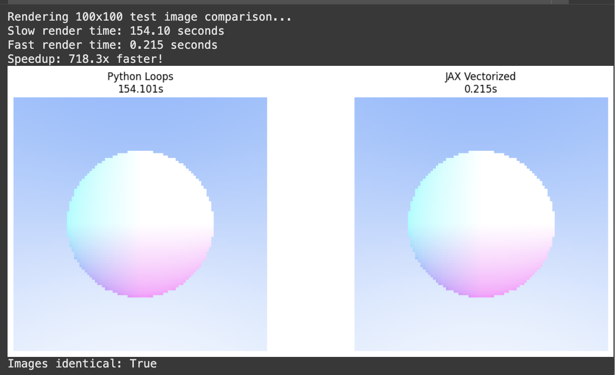
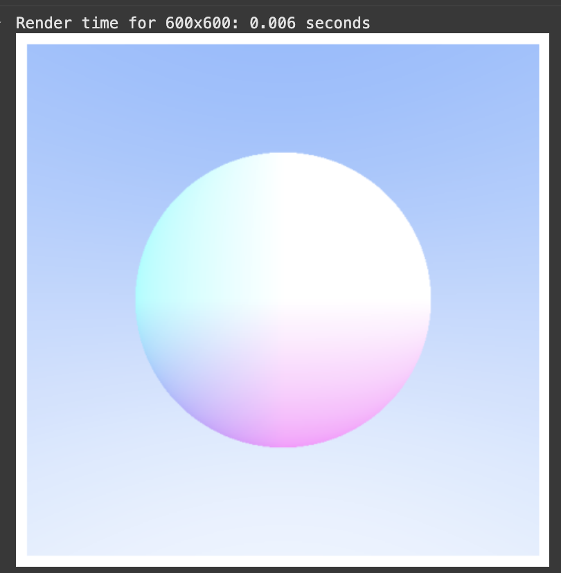
As you can see, JAX is much more efficient than Python loops. The slow version treats each pixel as a separate Python function call whereas the fast version lets JAX see the entire computation at once, enabling vectorization across all pixels simultaneously by leverage vmap. Even if you beef up the dimensions, JAX is still very fast.
Part 2: Multiple Spheres & Diffuse
Roughly covers the rest of Ch. 6: Multiple Objects and Ch. 9: Diffuse materials
Multiple Objects
Now we need to extend our one-sphere-wonder ray tracer to handle a scene with multiple spheres.
Traditional ray tracers loop through each sphere sequentially (i.e. test sphere 1, then sphere 2, then sphere 3) until you find the closest hit. However, JAX offers massive speedups by testing all spheres simultaneously with vmap, then find the minimum distance. Whether you have 5 spheres or 500, it’s still just one parallel operation — meaning the performance difference is quite noticeable as scenes get more complex.
def scene_intersect(ray_origin, ray_direction, centers, radii, material_ids):
  """Test ray against ALL spheres simultaneously"""
  intersect_all = vmap(ray_sphere_intersect, in_axes=(None, None, 0, 0))
  hits, ts, hit_points, normals = intersect_all(
      ray_origin, ray_direction,
      centers, radii
  )

  # Find closest valid hit (smallest positive t value)
  valid_ts = jnp.where(hits, ts, jnp.inf)
  closest_idx = jnp.argmin(valid_ts) # index of closest sphere

  t = valid_ts[closest_idx]
  p = hit_points[closest_idx]
  normal = normals[closest_idx]
  material_id = material_ids[closest_idx]
  hit = jnp.isfinite(t)

  return hit, t, p, normal, material_id
Diffuse Materials
When light hits a diffuse surface, rays scatter randomly in all directions - this creates the soft, natural lighting you see in real life. Thus, to implement diffuse surfaces (i.e. matte) we have to implement the ability to generate arbitrary random vectors.
In Rust, random number generation is simple, and NumPy natively supports PNRG using the numpy.random module, which is based on a global state and can be seeded deterministically.
However, JAX has more constraints. The desired PRNG properties are (1) reproducibility, (2) parallelizability, and (3) vectorizability.
NumPy’s PNRG is not parallelizable or vectorizable – but it doesn’t matter because NumPy always evaluates code in the order defined by the Python interpreter. However, JAX’s efficient execution relies on the JIT compiler’s ability to freely reorder, elide, and fuse operations in our functions. In multi-device environments, we also want to avoid needing to synchronize global state.
JAX uses explicit random state via a random key:
from jax import random
key = random.key(42)
The caveat here is that random functions consume the key but don’t modify it: if you use the same key, you will get the same sample output. If you want randomness in JAX, never re-use keys!
Additionally:
“JAX uses a modern Threefry counter-based PRNG that’s splittable. That is, its design allows us to fork the PRNG state into new PRNGs for use with parallel stochastic generation. In order to generate different and independent samples, you must split() the key explicitly before passing it to a random function. jax.random.split() is a deterministic function that converts one key into several independent (in the pseudorandomness sense) keys.” Read more here.
We use jax.random.split to ensure reproducible results while maintaining the mathematical purity that enables vectorization. Traditional imperative random number generators would break JAX’s ability to parallelize across pixels.
def random_unit_vector_jax(rng_key):
    """Generate random unit vector for diffuse scattering"""
    # Random point in unit sphere, then normalize
    key1, key2, key3 = jax.random.split(rng_key, 3)
    x = jax.random.normal(key1)
    y = jax.random.normal(key2)
    z = jax.random.normal(key3)
    vec = jnp.array([x, y, z])
    return normalize(vec)
Now we can implement recursive ray coloring with diffuse material.
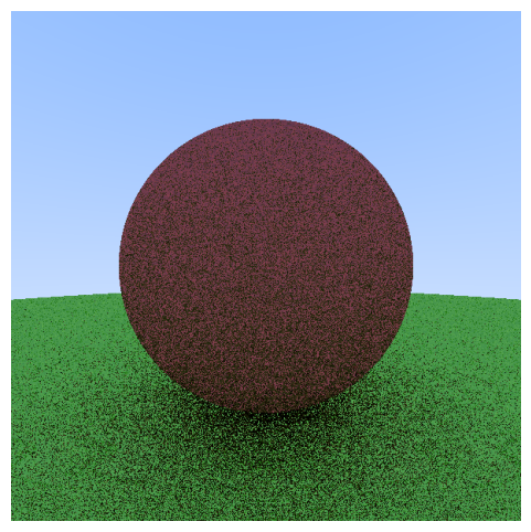
Albedo is the material’s intrinsic color — how much of each color channel (red, green, blue) the surface reflects. An albedo of [0.7, 0.3, 0.3] means the material reflects 70% of red light but only 30% of green and blue, making it appear reddish.
When a ray hits a diffuse surface, it scatters in a random direction. The final color is the material’s albedo multiplied by the color of light coming from that random direction, which requires tracing another ray recursively. This is what creates realistic indirect lighting where surfaces illuminate each other.
def trace_pixel_scene(i, j, image_width, image_height, centers, radii, material_ids, material_albedos, rng_key):
  """Cast a ray through pixel (i,j) and return its color using diffuse materials"""
  ray_origin, ray_direction = camera_get_ray(i, j, image_width, image_height)
  return ray_color_diffuse(ray_origin, ray_direction, centers, radii, material_ids, material_albedos, rng_key)

trace_pixel_scene_jit = jit(trace_pixel_scene, static_argnums=(2, 3))

def ray_color_diffuse(ray_origin, ray_direction, centers, radii, material_ids, material_albedos, rng_key, depth=0, max_depth=8):
  """Recursively trace rays with Lambertian (diffuse) material scattering"""
  if depth >= max_depth:
        return jnp.array([0.0, 0.0, 0.0])

  hit, t, p, normal, material_id = scene_intersect(ray_origin, ray_direction, centers, radii, material_ids)
  albedo = material_albedos[material_id]

  # Lambertian scattering
  key1, key2 = jax.random.split(rng_key)
  scatter_direction = normalize(normal + random_unit_vector_jax(key1))

  # Recursive bounce
  bounced_color = ray_color_diffuse(
      p + 0.001 * normal, scatter_direction, centers, radii, material_ids, material_albedos, key2, depth + 1, max_depth
  )

  # Sky color
  unit_direction = normalize(ray_direction)
  a = 0.5 * (unit_direction[1] + 1.0)
  sky_color = (1.0 - a) * jnp.array([1.0, 1.0, 1.0]) + a * jnp.array([0.5, 0.7, 1.0])

  sphere_color = albedo * bounced_color
  return jnp.where(hit, sphere_color, sky_color)
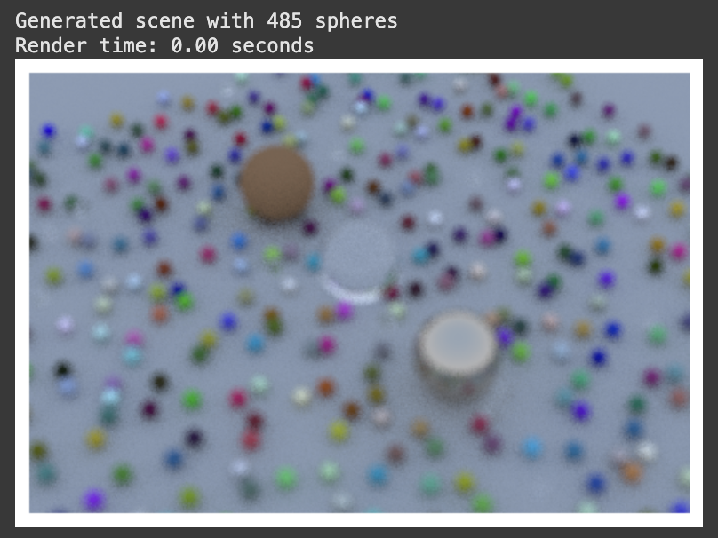
I rewrote the render_image() function and made a create_diffuse_scene() which resulted in:
Part 3: Advanced Camera and Smoothing
Covers Ch. 12: Positionable Camera, Ch. 13: Defocus Blur, and Ch. 8: Antialiasing
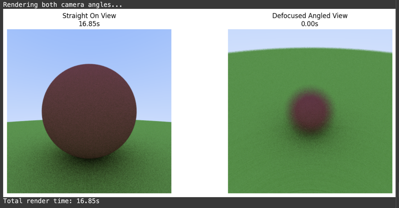
Positional Camera & Defocus Blur
Now we can start to add some more flexibility with our camera:
-
Positionable POV: Instead of rays starting from a single point, we can position our camera anywhere in 3D space and point it in any direction. This lets us create more interesting viewpoints (e.g. looking up at spheres, angled shots, placing the camera inside the scene). We
-
Defocus Blur (Depth of Field): Real cameras have lenses with finite apertures, creating depth of field effects where objects at the focal distance are sharp while nearer/farther objects appear blurry. We simulate this by randomly sampling ray origins from a small disk (the aperture) rather than a single point, then focusing all rays toward the same point on the focal plane.
Both of these features are just some added ray calculations and additional sampling per pixel in our main camera function such as vfov is adjustable field of view, lookfrom is camera at origin, and lookat is looking down negative Z axis.
def create_positionable_camera(image_width, image_height, vfov, lookfrom, lookat, vup, defocus_angle, focus_dist):
  aspect_ratio = image_width / image_height

  focal_length = len(lookfrom - lookat)
  theta = jnp.deg2rad(vfov)
  h = jnp.tan(theta/2)
  viewport_height = 2.0 * h * focus_dist
  viewport_width = viewport_height * (image_width / image_height)

  camera_center = lookfrom

  w = normalize(lookfrom - lookat)
  u = normalize(jnp.cross(vup, w))
  v = jnp.cross(w, u)

  viewport_u = viewport_width * u
  viewport_v = viewport_height * -v

  pixel_delta_u = viewport_u / image_width
  pixel_delta_v = viewport_v / image_height

  viewport_upper_left = (camera_center -
                        focus_dist * w -
                        viewport_u/2 - viewport_v/2)
  pixel00_loc = viewport_upper_left + 0.5 * (pixel_delta_u + pixel_delta_v)

  # calculate camera defocus disk basis vectors
  defocus_radius = focus_dist * jnp.tan(jnp.deg2rad(defocus_angle / 2))
  defocus_disk_u = u * defocus_radius
  defocus_disk_v = v * defocus_radius

  return image_width, image_height, aspect_ratio, camera_center, pixel00_loc, pixel_delta_u, pixel_delta_v, defocus_disk_u, defocus_disk_v
def random_in_unit_disk_jax(key):
     """Fixed random point in unit disk"""
    # Generate random angle and radius
    key1, key2 = jax.random.split(key, 2)
    angle = jax.random.uniform(key1, minval=0.0, maxval=2.0 * jnp.pi)
    r = jnp.sqrt(jax.random.uniform(key2, minval=0.0, maxval=1.0))  # sqrt for uniform distribution

    # Convert to cartesian
    x = r * jnp.cos(angle)
    y = r * jnp.sin(angle)
    return jnp.array([x, y, 0.0])

def defocus_disk_sample(key, camera_center, defocus_disk_u, defocus_disk_v):
    """Returns a random point in the camera defocus disk"""
    p = random_in_unit_disk_jax(key)
    return camera_center + p[0] * defocus_disk_u + p[1] * defocus_disk_v
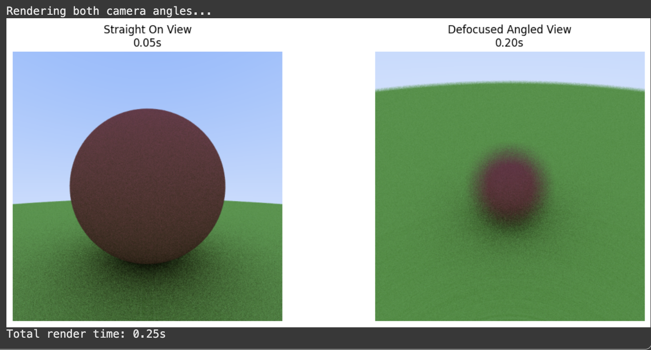
Anti-aliasing
Anti-aliasing smooths out the jagged “staircase” edges you get when rendering 3D scenes onto a pixel grid.
Basic ray tracing shoots one ray through each pixel’s center: the pixel is either fully “sphere” or fully “sky” with no middle ground. This creates harsh, blocky edges where objects meet the background.
Instead of one ray per pixel, we shoot multiple rays at random positions within each pixel and average their colors. If 3 out of 4 sample rays hit the sphere, that pixel becomes 75% sphere color + 25% sky color, creating smooth gradients along edges.
Anti-aliasing dramatically increases the computational load — instead of 360k rays for a 600x600 image, you might need 3.6 million rays (10 samples per pixel). However, JAX’s vectorization handles this explosion of parallel computation naturally so we can still achieve smooth renders without taking massive performance hits.
def camera_get_ray_antialiased(i, j, image_width, image_height, vfov, lookfrom, lookat, vup, defocus_angle, focus_dist, rng_key):
    """Generate a ray with random sampling within the pixel for anti-aliasing"""
    # Construct a camera ray originating from the defocus disk and directed at a randomly sampled point around the pixel location i, j.
    _, _, _, camera_center, pixel00_loc, pixel_delta_u, pixel_delta_v, defocus_disk_u, defocus_disk_v = create_positionable_camera(image_width, image_height, vfov, lookfrom, lookat, vup, defocus_angle, focus_dist)

    key1, key2, key3 = jax.random.split(rng_key, 3)

    # Add random offset within pixel bounds
    offset_u = jax.random.uniform(key1, minval=-0.5, maxval=0.5)
    offset_v = jax.random.uniform(key2, minval=-0.5, maxval=0.5)

    pixel_center = pixel00_loc + ((i + offset_u) * pixel_delta_u) + ((j + offset_v) * pixel_delta_v)

    ray_origin = jnp.where(defocus_angle <= 0, camera_center, defocus_disk_sample(key3, camera_center, defocus_disk_u, defocus_disk_v))
    ray_direction = normalize(pixel_center - camera_center)

    return ray_origin, ray_direction
We update the trace_pixel() and render_scene() functions to use camera_get_ray_antialiased(), e.g.:
def trace_pixel_antialiased(i, j, image_width, image_height, vfov, lookfrom, lookat, vup, defocus_angle, focus_dist, centers, radii, material_ids, material_albedos, rng_key, samples_per_pixel):
  """Trace a pixel with multiple samples for anti-aliasing"""

  # Generate keys for each sample
  sample_keys = jax.random.split(rng_key, samples_per_pixel * 2)
  camera_keys = sample_keys[:samples_per_pixel]
  ray_keys = sample_keys[samples_per_pixel:]

  def trace_single_sample(camera_key, ray_key):
      ray_origin, ray_direction = camera_get_ray_antialiased(i, j, image_width, image_height, vfov, lookfrom, lookat, vup, defocus_angle, focus_dist, camera_key)
      return ray_color_diffuse(ray_origin, ray_direction, centers, radii, material_ids, material_albedos, ray_key)

  # Vectorize over all samples
  trace_samples = vmap(trace_single_sample)
  sample_colors = trace_samples(camera_keys, ray_keys)

  # Average the samples
  return jnp.mean(sample_colors, axis=0)
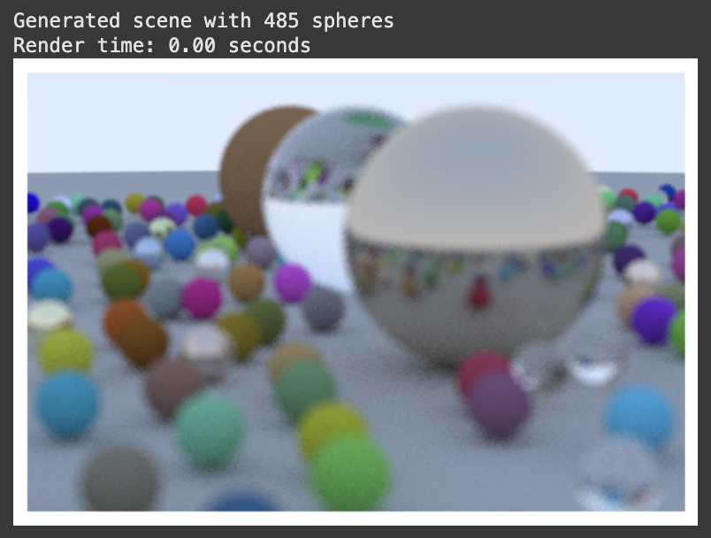
If I am up the defocus blur on the zoomed in image, we get:
Part 4: Final Render
Roughly covers Ch. 10: Metal, Ch. 11: Dielectrics, and Ch. 14’s Final Render.
Metals & Dielectrics
Now we add two more materials that interact with light much differently than diffuse surfaces: (1) metal and (2) dielectric.
Metals reflect light in a specific direction rather than scattering randomly. The reflect function implements perfect mirror reflection using the formula v - 2(v·n)n, where the incident ray bounces off at the same angle it came in. We add a “fuzz” parameter that slightly randomizes the reflection direction, simulating surface roughness (polished meta has 0 fuzz).
Glass both reflects and refracts light depending on the viewing angle. The refract function implements Snell’s law to bend light as it passes through the material boundary. The reflectance function calculates Fresnel reflectance: at shallow angles, glass acts more like a mirror, while at steep angles it’s more transparent. We randomly choose between reflection and refraction based on these physical probabilities.
# Reflected ray direction: v + 2b where b is the vector projection of v onto n
def reflect(incident, normal):
  return incident - 2.0 * jnp.dot(incident, normal) * normal

def refract(uv, normal, etai_over_etat):
  """Calculate refraction direction using Snell's law"""
  cos_theta = jnp.minimum(-jnp.dot(uv, normal), 1.0)
  r_out_perp = etai_over_etat * (uv + cos_theta * normal)
  r_out_parallel = -jnp.sqrt(jnp.abs(1.0 - jnp.dot(r_out_perp, r_out_perp))) * normal
  return r_out_perp + r_out_parallel

def reflectance(cosine, ref_idx):
  r0 = (1.0 - ref_idx) / (1.0 + ref_idx)
  r0 = r0 * r0
  return r0 + (1.0 - r0) * jnp.power(1.0 - cosine, 5.0)
Each material type requires different physics calculations, random decisions, and careful normal vector handling (especially for glass, where rays can enter or exit the material).
Unfortunately, JAX’s constraints for dynamic control flow means the jnp.where conditionals get a bit gnarly in terms of readability (not to mention the PNRG key mangement)…
def ray_color_materials(ray_origin, ray_direction, centers, radii, material_ids, material_data, rng_key, depth=0, max_depth=10):
  """Ray tracing with diffuse, metal, and glass materials"""
  if depth >= max_depth:
      return jnp.array([0.0, 0.0, 0.0])

  hit, t, p, normal, material_id = scene_intersect(ray_origin, ray_direction, centers, radii, material_ids)

  material_type = material_data['types'][material_id]
  albedo = material_data['albedos'][material_id]
  fuzz = material_data['fuzz'][material_id]
  refractive_index = material_data['refractive_indices'][material_id]

  # Split into many keys to avoid reuse
  key_diffuse, key_metal, key_glass_reflect, key_glass_random, key_recursive = jax.random.split(rng_key, 5)

  # Diffuse scattering
  diffuse_scatter = normal + random_unit_vector_jax(key_diffuse)
  near_zero = jnp.linalg.norm(diffuse_scatter) < 1e-8
  diffuse_scatter = jnp.where(near_zero, normal, diffuse_scatter)

  # Metal reflection
  reflected = reflect(normalize(ray_direction), normal)
  metal_scatter = reflected + fuzz * random_unit_vector_jax(key_metal)

  # Glass refraction/reflection
  front_face = jnp.dot(ray_direction, normal) < 0
  outward_normal = jnp.where(front_face, normal, -normal)
  eta_ratio = jnp.where(front_face, 1.0 / refractive_index, refractive_index)

  unit_direction = normalize(ray_direction)
  cos_theta = jnp.minimum(-jnp.dot(unit_direction, outward_normal), 1.0)
  sin_theta = jnp.sqrt(1.0 - cos_theta * cos_theta)

  cannot_refract = eta_ratio * sin_theta > 1.0

  should_reflect = cannot_refract | (jax.random.uniform(key_glass_random) < reflectance(cos_theta, eta_ratio))

  refracted_direction = refract(unit_direction, outward_normal, eta_ratio)
  reflected_direction = reflect(unit_direction, outward_normal)

  glass_scatter = jnp.where(should_reflect, reflected_direction, refracted_direction)

  # Choose scatter direction based on material type
  scatter_direction = jnp.where(
      material_type == 0, diffuse_scatter,
      jnp.where(material_type == 1, metal_scatter, glass_scatter)
  )

  metal_absorbed = (material_type == 1) & (jnp.dot(metal_scatter, normal) <= 0)

  ray_offset_normal = jnp.where(
      (material_type == 2) & ~should_reflect,  # Glass refraction
      -outward_normal,  # Offset into the material
      outward_normal    # Offset away from surface
  )

  bounced_color = ray_color_materials(
      p + 0.001 * ray_offset_normal, scatter_direction,
      centers, radii, material_ids, material_data,
      key_recursive, depth + 1, max_depth
  )

  # sky
  unit_direction_sky = normalize(ray_direction)
  a = 0.5 * (unit_direction_sky[1] + 1.0)
  sky_color = (1.0 - a) * jnp.array([1.0, 1.0, 1.0]) + a * jnp.array([0.5, 0.7, 1.0])

  material_albedo = jnp.where(material_type == 2, jnp.array([1.0, 1.0, 1.0]), albedo)
  sphere_color = material_albedo * bounced_color

  # metal absorption
  sphere_color = jnp.where(metal_absorbed, jnp.array([0.0, 0.0, 0.0]), sphere_color)

  return jnp.where(hit, sphere_color, sky_color)
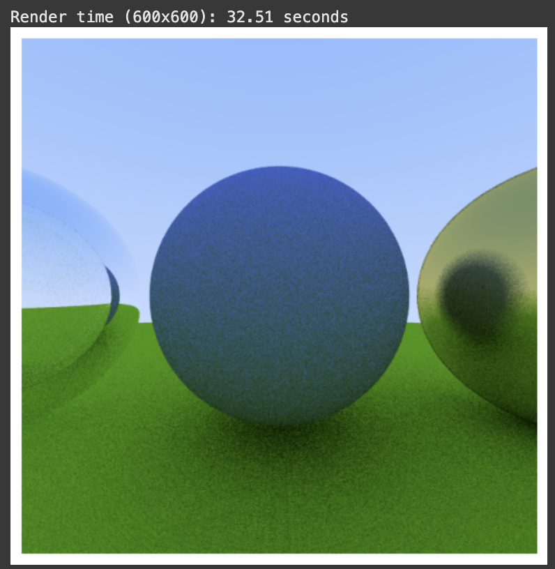
Now we can render a four-sphere scene (three balls + the ground) with all different materials. The left glass sphere is an air bubble, the middle is a diffuse sphere, and the right is a metal sphere – just like the Ray Tracer tutorial.
def create_all_materials_scene():
  centers = jnp.array([
      [-1.1, 0.0, -1.0],     # Left glass sphere
      [0.0, -0., -1.0],      # Center diffuse sphere
      [1.1, 0.0, -1.0],      # Right metal sphere
      [0.0, -100.5, -1.0],   # Ground
  ])

  radii = jnp.array([0.5, 0.45, 0.5, 100.0])
  material_ids = jnp.array([0, 1, 2, 3])

  material_data = {
      'types': jnp.array([2, 0, 1, 0]),  # glass, diffuse, metal, diffuse
      'albedos': jnp.array([
          [1.0, 1.0, 1.0],   # Glass (no attenuation)
          [0.4, 0.5, 0.8],   # Blue diffuse sphere
          [0.9, 0.8, 0.4],   # Gold metal sphere
          [0.5, 0.8, 0.0],   # Green ground
      ]),
      'fuzz': jnp.array([0.0, 0.0, 0.2, 0.0]),  # Some fuzz on metal
      'refractive_indices': jnp.array([1.0/1.33, 1.0, 1.0, 1.0])
  }

  return centers, radii, material_ids, material_data
JAX lets us naturally compose two levels of parallelization. First, we vmap over multiple samples per pixel (for anti-aliasing), then vmap over all pixels in the image.
The JIT compiler creates highly optimized parallel code that can be scaled across CPU cores or GPU threads automatically. For a 600x600 image with 16 samples per pixel, we’re processing 5.76 million rays simultaneously.
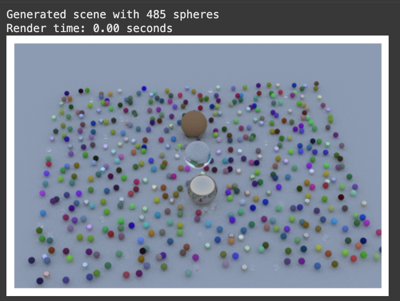
After making some new trace_pixel() and render() wrapper functions, we get:
A Final Render
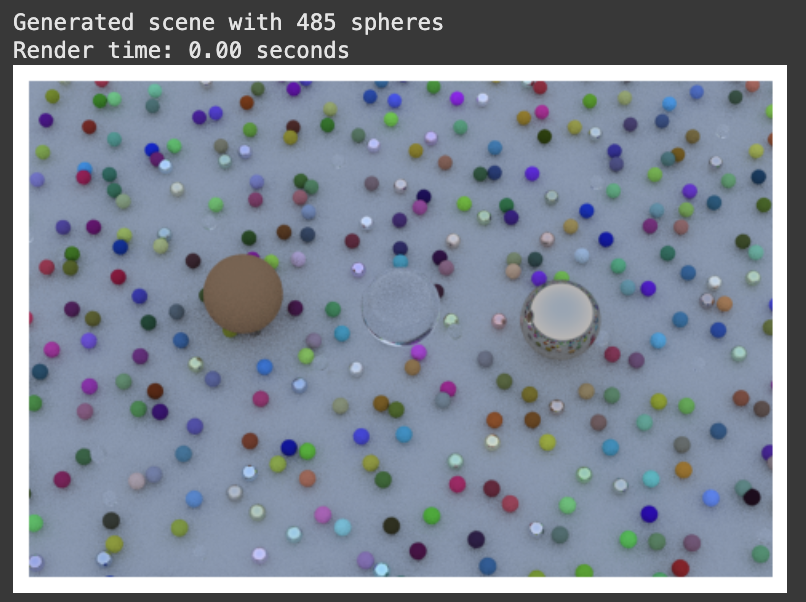
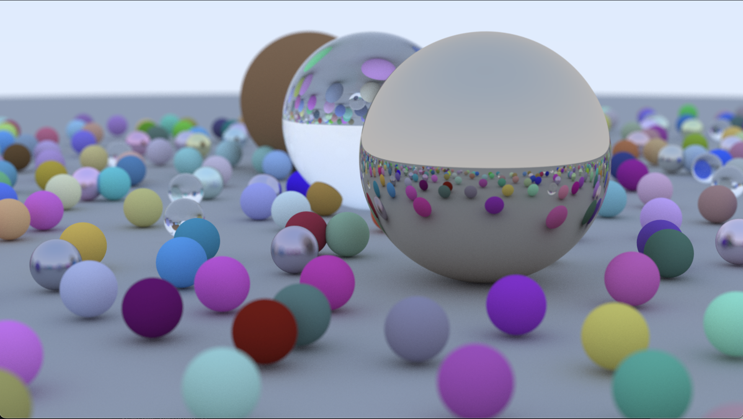
Now it’s time create the iconic final scene from the tutorial with lots and lots of spheres!! (The details of create_hella_balls_scene() aren’t really relevant – the main point is that there are lots of balls with lots of different materials. I also had to implement some batching to get around the memory constraints.)
I added some simple gamma correction (gamma = 2.2, so we take square root for approximate 2.0) to the rendering pipeline for better coloring, which can be done using this line: jnp.sqrt(jnp.clip(linear_color, 0.0, 1.0)). With max_depth = 10 and samples_per_pixel = 12, here’s a comparison of before and after gamma correction:
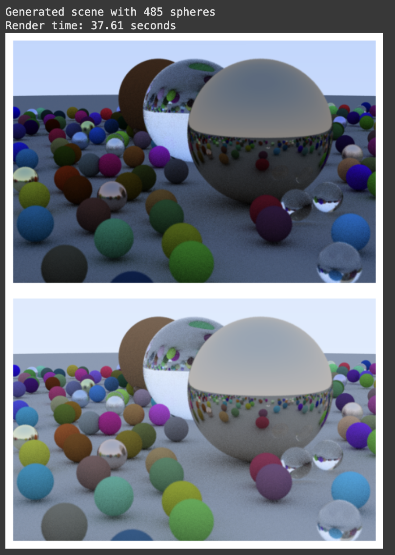
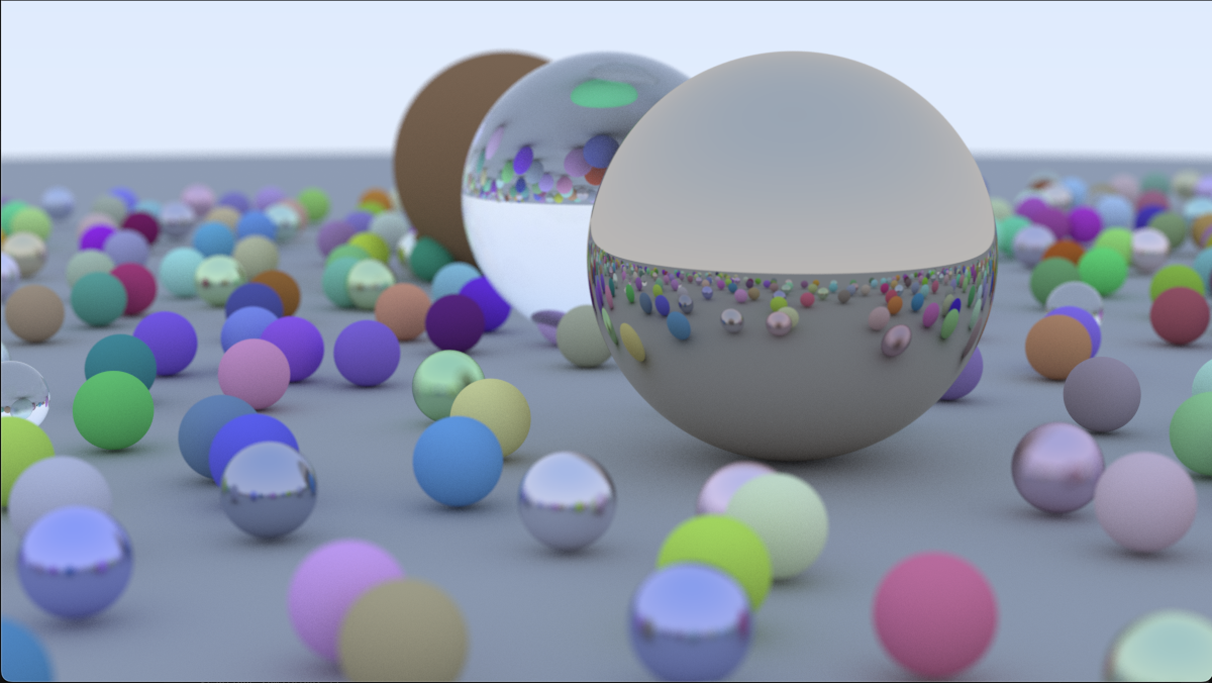
With max_depth = 10 and samples_per_pixel = 500 after gamma correction… VOILA!!
Subsequent renders are fast because JAX caches the JIT-compiled functions. As long as you keep the same image dimensions (static arguments), changing camera position, materials, or scene geometry doesn’t trigger recompilation - JAX reuses the optimized machine code.
Speed comes from: (a) no recompilation for non-static argument changes, (b) vectorized operations processing millions of rays in parallel, and (c) XLA optimizations like operation fusion and memory layout optimization.
For reference, these image generated in Rust on my machine took 1244.58 seconds (a little over 20 minutes) and 1236.66 seconds. The first had max_depth=20 and the second was max_depth=10 (both samples_per_pixel = 500). (The Rust version looks slightly different, maybe a bit more “high quality”, but I think it’s just due to some small implementation details like PNRG and different epsilon calculations.)
Again if you want to play around for yourself, here is the Colab!